Plotting data on the graph is like looking at a bunch of stars. They all look the same and the data is difficult to interpret. What if there was a method to colour the stars?

Red stars are associated with red flowers and blue stars are associated with yellow flowers

Cluster analysis groups observations into subsets based on the similarity of responses on various relational variables, called clusters. The data is plotted on a graph and different clusters are coloured and separated to make sense of data. Today we will be using the same data set (NESARC wave 1) as the previous two examples: 1, 2

The target will be alcohol intake (≥12 drinks in 12 months, lower score = higher intake) and the cluster variables are again as follows:
1. SEX
2. HISPANIC OR LATINO ORIGIN (S1Q1C)
3. “AMERICAN INDIAN OR ALASKA NATIVE” CHECKED IN MULTIRACE CODE (S1Q1D1)
4. “ASIAN” CHECKED IN MULTIRACE CODE (S1Q1D2)
5. “BLACK OR AFRICAN AMERICAN” CHECKED IN MULTIRACE CODE (S1Q1D3)
6. “NATIVE HAWAIIAN OR OTHER PACIFIC ISLANDER” CHECKED IN MULTIRACE CODE (S1Q1D4)
7. “WHITE” CHECKED IN MULTIRACE CODE (S1Q1D5)
8. NUMBER OF CHILDREN EVER HAD, INCLUDING ADOPTIVE, STEP AND FOSTER CHILDREN (S1Q5A)
9. PRESENT SITUATION INCLUDES WORKING FULL TIME (35+ HOURS A WEEK) (S1Q7A1)
10. PERSONALLY RECEIVED FOOD STAMPS IN LAST 12 MONTHS (S1Q14A)

The syntax is as follows:

 -- coding: UTF-8 --
 from pandas import Series, DataFrame
 from pandas import Series, DataFrame
 import pandas as pd
 import numpy as np
 import matplotlib.pylab as plt
 from sklearn.cross_validation import train_test_split
 from sklearn import preprocessing
 from sklearn.cluster import KMeans
 import os
 Remember to replace file directory with the active folder
 os.chdir("file directory")
 Load the dataset
 data = pd.read_csv("nesarc_pds.csv", low_memory=False)
 upper-case all DataFrame column names
 data.columns = map(str.upper, data.columns)
 data_clean = data.dropna()
 Clustering Variables
 cluster = data_clean[['SEX','S1Q1C','S1Q1D1','S1Q1D2','S1Q1D3','S1Q1D4','S1Q1D5','S1Q5A','S1Q7A1','S1Q14A']]
 cluster.describe()
 target = data_clean.S2AQ2
 standardize clustering variables to have mean=0 and sd=1
 clustervar=cluster.copy()
 clustervar['SEX']=preprocessing.scale(clustervar['SEX'].astype('float64'))
 clustervar['S1Q1C']=preprocessing.scale(clustervar['S1Q1C'].astype('float64'))
 clustervar['S1Q1D1']=preprocessing.scale(clustervar['S1Q1D1'].astype('float64'))
 clustervar['S1Q1D2']=preprocessing.scale(clustervar['S1Q1D2'].astype('float64'))
 clustervar['S1Q1D3']=preprocessing.scale(clustervar['S1Q1D3'].astype('float64'))
 clustervar['S1Q1D4']=preprocessing.scale(clustervar['S1Q1D4'].astype('float64'))
 clustervar['S1Q1D5']=preprocessing.scale(clustervar['S1Q1D5'].astype('float64'))
 clustervar['S1Q5A']=preprocessing.scale(clustervar['S1Q5A'].astype('float64'))
 clustervar['S1Q7A1']=preprocessing.scale(clustervar['S1Q7A1'].astype('float64'))
 clustervar['S1Q14A']=preprocessing.scale(clustervar['S1Q14A'].astype('float64'))
 split data into train and test sets
 clus_train, clus_test = train_test_split(clustervar, test_size=.3, random_state=111)
 k-means cluster analysis for 1-9 clusters
 from scipy.spatial.distance import cdist
 clusters=range(1,10)
 meandist=[]
 for k in clusters:
 model=KMeans(n_clusters=k)
 model.fit(clus_train)
 clusassign=model.predict(clus_train)
 meandist.append(sum(np.min(cdist(clus_train, model.cluster_centers_, 'euclidean'), axis=1))
 / clus_train.shape[0])
 Plot
 plt.plot(clusters, meandist)
 plt.xlabel('Number of clusters')
 plt.ylabel('Average distance')
 plt.title('Selecting k with the Elbow Method')
 plt.show()
 2 cluster solution
 model2=KMeans(n_clusters=2)
 model2.fit(clus_train)
 clusassign=model2.predict(clus_train)
 plot clusters
 from sklearn.decomposition import PCA
 pca_2 = PCA(2)
 plot_columns = pca_2.fit_transform(clus_train)
 plt.scatter(x=plot_columns[:,0], y=plot_columns[:,1], c=model2.labels_,)
 plt.xlabel('Canonical variable 1')
 plt.ylabel('Canonical variable 2')
 plt.title('Scatterplot of Canonical Variables for 2 Clusters')
 plt.show()
 merge cluster assignment with clustering variables to examine cluster variable means by cluster
 clus_train.reset_index(inplace=True)
 cluslist=list(clus_train['index'])
 labels=list(model2.labels_)
 newlist=dict(zip(cluslist, labels))
 newlist
 newclus=DataFrame.from_dict(newlist, orient='index')
 newclus
 newclus.columns = ['cluster']
 now do the same for the cluster assignment variable
 newclus.reset_index(inplace=True)
 merged_train=pd.merge(clus_train, newclus, on='index')
 merged_train.head(n=100)
 merged_train.cluster.value_counts()
 calculate clustering variable means by cluster
 clustergrp = merged_train.groupby('cluster').mean()
 print ("Clustering variable means by cluster")
 print(clustergrp)
 first have to merge ALC with clustering variables and cluster assignment data
 alc_data=data_clean['S2AQ2']
 split GPA data into train and test sets
 alc_train, alc_test = train_test_split(alc_data, test_size=.3, random_state=111)
 alc_train1=pd.DataFrame(alc_train)
 alc_train1.reset_index(inplace=True)
 merged_train_all=pd.merge(alc_train1, merged_train, on='index')
 sub1 = merged_train_all[['S2AQ2', 'cluster']].dropna()
 import statsmodels.formula.api as smf
 import statsmodels.stats.multicomp as multi
 alcmod = smf.ols(formula='S2AQ2 ~ C(cluster)', data=sub1).fit()
 print (alcmod.summary())
 print ('Means for Higher Alcohol Intake By Cluster')
 m1= sub1.groupby('cluster').mean()
 print (m1)
 print ('standard deviations for ALC by cluster')
 m2= sub1.groupby('cluster').std()
 print (m2)
 mc1 = multi.MultiComparison(sub1['S2AQ2'], sub1['cluster'])
 res1 = mc1.tukeyhsd()
 print(res1.summary())

A series of k-means cluster analyses were conducted on the training data specifying k=1-9 clusters, using Euclidean distance. The elbow curve demonstrates the variance in clustering variables and shows sharp turning point at 2 clusters, although 4-cluster-analysis is also suggested. For the purpose of simplicity, 2-cluster-analysis is obtained although the number of clusters should be determined by canonical discriminant analyses.

The second graph is a plot of the first two canonical variables for the clustering variables by cluster. This shows that the clusters are distinct with little overlap.

The output is as follows:

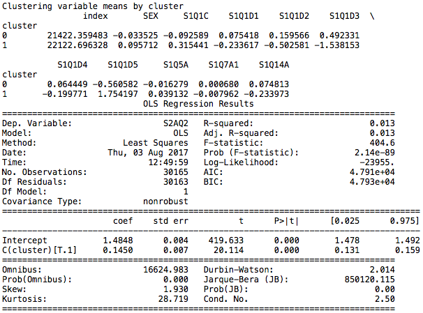
The clusters are named Cluster 0 and Cluster 1.

Cluster 0
Main characteristics include being white, having fewer children and being employed.

Cluster 1
Main characteristics include being black, having more children, being unemployed and receiving food stamps.

The difference between the groups is determined to be significant and cluster 0 is associated with higher alcohol intake, having a lower number assigned according to the codebook.

As per the previous results, the cluster consisting of whites with fewer children, being employed and not having received food stamps suggests that it is the availability of resources that determines higher alcohol intake. However, having more alcohol does not indicate dependence and having 12 drinks in 12 months remains acceptable by societal standards.