Lasso regression (AKA Penalized regression method) is often used to select a subset of variables. It is a supervised machine learning method which stands for “Least Absolute Selection and Shrinkage Operator”.

The shrinkage process identifies the variables most strongly associated with the selected target variable. We will be using the same target and explanatory variables from the post on Random Forests. This helps us compare the different ways to select important variables that affect the target.

The variables are again:
1. SEX
2. HISPANIC OR LATINO ORIGIN (S1Q1C)
3. “AMERICAN INDIAN OR ALASKA NATIVE” CHECKED IN MULTIRACE CODE (S1Q1D1)
4. “ASIAN” CHECKED IN MULTIRACE CODE (S1Q1D2)
5. “BLACK OR AFRICAN AMERICAN” CHECKED IN MULTIRACE CODE (S1Q1D3)
6. “NATIVE HAWAIIAN OR OTHER PACIFIC ISLANDER” CHECKED IN MULTIRACE CODE (S1Q1D4)
7. “WHITE” CHECKED IN MULTIRACE CODE (S1Q1D5)
8. NUMBER OF CHILDREN EVER HAD, INCLUDING ADOPTIVE, STEP AND FOSTER CHILDREN (S1Q5A)
9. PRESENT SITUATION INCLUDES WORKING FULL TIME (35+ HOURS A WEEK) (S1Q7A1)
10. PERSONALLY RECEIVED FOOD STAMPS IN LAST 12 MONTHS (S1Q14A)

The target is set to “DRANK AT LEAST 12 ALCOHOLIC DRINKS IN LAST 12 MONTHS”Data were randomly split into a training set that included 70% of the observations (N=3201) and a test set that included 30% of the observations (N=1701).

Data were randomly split into a training set that included 70% of the observations and a test set that included 30% of the observations. The syntax is as follows:

[code language="python"]
 -- coding: UTF-8 --
 from pandas import Series, DataFrame
 import pandas as pd
 import os
 import numpy as np
 import matplotlib.pylab as plt
 from sklearn.cross_validation import train_test_split
 from sklearn.linear_model import LassoLarsCV
 Remember to replace file directory with the active folder
 os.chdir("file directory")
 Load the dataset
 data = pd.read_csv("nesarc_pds.csv", low_memory=False)
 upper-case all DataFrame column names
 data.columns = map(str.upper, data.columns)
 data_clean = data.dropna()
 Split into training and testing sets
 predvar = data_clean[['SEX','S1Q1C','S1Q1D1','S1Q1D2','S1Q1D3','S1Q1D4','S1Q1D5','S1Q5A','S1Q7A1','S1Q14A']]
 target = data_clean.S2AQ2
 standardize predictors to have mean=0 and sd=1
 predictors=predvar.copy()
 from sklearn import preprocessing
 scaling every variable
 predictors['SEX']=preprocessing.scale(predictors['SEX'].astype('float64'))
 predictors['S1Q1C']=preprocessing.scale(predictors['S1Q1C'].astype('float64'))
 predictors['S1Q1D1']=preprocessing.scale(predictors['S1Q1D1'].astype('float64'))
 predictors['S1Q1D2']=preprocessing.scale(predictors['S1Q1D2'].astype('float64'))
 predictors['S1Q1D3']=preprocessing.scale(predictors['S1Q1D3'].astype('float64'))
 predictors['S1Q1D4']=preprocessing.scale(predictors['S1Q1D4'].astype('float64'))
 predictors['S1Q1D5']=preprocessing.scale(predictors['S1Q1D5'].astype('float64'))
 predictors['S1Q5A']=preprocessing.scale(predictors['S1Q5A'].astype('float64'))
 predictors['S1Q7A1']=preprocessing.scale(predictors['S1Q7A1'].astype('float64'))
 predictors['S1Q14A']=preprocessing.scale(predictors['S1Q14A'].astype('float64'))
 split data into train and test sets
 pred_train, pred_test, tar_train, tar_test = train_test_split(predictors, target,
 test_size=.3, random_state=123)
 specify the lasso regression model
 model=LassoLarsCV(cv=10, precompute=False).fit(pred_train,tar_train)
 print variable names and regression coefficients
 dict(zip(predictors.columns, model.coef_))
 plot coefficient progression
 m_log_alphas = -np.log10(model.alphas_)
 ax = plt.gca()
 plt.plot(m_log_alphas, model.coef_path_.T)
 plt.axvline(-np.log10(model.alpha_), linestyle='--', color='k',
 label='alpha CV')
 plt.ylabel('Regression Coefficients')
 plt.xlabel('-log(alpha)')
 plt.title('Regression Coefficients Progression for Lasso Paths')
 plot mean square error for each fold
 m_log_alphascv = -np.log10(model.cv_alphas_)
 plt.figure()
 plt.plot(m_log_alphascv, model.cv_mse_path_, ':')
 plt.plot(m_log_alphascv, model.cv_mse_path_.mean(axis=-1), 'k',
 label='Average across the folds', linewidth=2)
 plt.axvline(-np.log10(model.alpha_), linestyle='--', color='k',
 label='alpha CV')
 plt.legend()
 plt.xlabel('-log(alpha)')
 plt.ylabel('Mean squared error')
 plt.title('Mean squared error on each fold')
 MSE from training and test data
 from sklearn.metrics import mean_squared_error
 train_error = mean_squared_error(tar_train, model.predict(pred_train))
 test_error = mean_squared_error(tar_test, model.predict(pred_test))
 print ('training data MSE')
 print(train_error)
 print ('test data MSE')
 print(test_error)
 R-square from training and test data
 rsquared_train=model.score(pred_train,tar_train)
 rsquared_test=model.score(pred_test,tar_test)
 print ('training data R-square')
 print(rsquared_train)
 print ('test data R-square')
 print(rsquared_test)
 [/code]

The output is as follows.

As you can see, the three variables with the highest weights in order are gender, having a full-time job and having fewer children. The variables with more weights are similar to the results using the random forest. All 3 variables show positive regression coefficients as you can see in the first graph below, indicated by blue, yellow and magenta respectively.

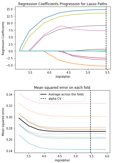
The second graph shows that prediction error decreases as more variables are added to the model. However, as more variables are added, the reduction in mean squared error became negligible. A model with too few predictors has a risk of being under-chosen and a model with too many predictors has a risk of being over-fitted.

It is interesting to know that people with full-time jobs and fewer children tend to drink more. Perhaps this is due to having more resources.